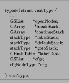
For the extraction of the CFG (control flow graph), we add some fields to the visitType structure. Those structures are shown on Figure 11.
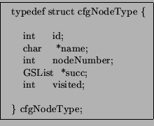
The openNodeList contains nodes of the type cfgNodeType (see Figure 12). A node has an id which is the number of the basic block. In this paper, we will consider as basic block each single expression or as a delimiter. For example, when we are in a "while" statement, we first create an empty block just to indicate that we start the extraction of the "while" statement. This is done to simplify the extraction of the CFG. A name is associated with the kind of the node (DO_BEGIN, DO_COND, DO_END, ...). We also find an integer nodeNumber. This integer contains the number of the corresponding node in the abstract syntax tree (ASG). Finally, the list succ contains the successor of the basic bloc. To return from there with the openNodes, this list contains a whole of nodes which we are calculating their successors.
We add many stacks in the structure to treat the embedded strucutre. The "goto" is a different case. For this one, we store in a list an item which has two fields, one is a pointer to the node corresponding to the "goto" and, the second is the label node number pointed by the "goto" in the ASG. In the same time, we maintain a hash table for the label. The key is the label node number and the cell is a pointer to the corresponding label in the CFG.
As we said, there is one CFG per functions, thus, we have a list of CFG (GSLIST *cfgs), and, each node of the list refers to a CFG (cfgNodeType *cfg).
Now, we can explain the differents algorithms used by gasta to produce a CFG using our visitor.
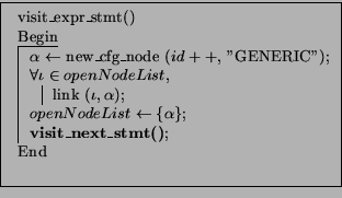
The first one (shown on Figure 13) and the simplest is used when visiting an expression statement. As we consider an expression as a basic block, we just need to link all nodes found inside the openNodeList list to the current basic block and then, update the list of open nodes with the current basic block.
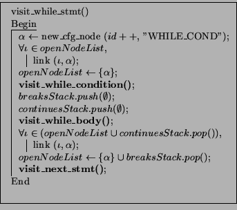
The second one is shown on Figure 14. The first step is the creation of a node which represents the begining of a "while" statement. After the creation, we link nodes in the openNodeList to the block we just created. After that, the openNodeList has only this node. Before visiting the body of the "while" statement, we push an empty set on both stacks (breaks and continues stack). As soon as the visit of the "while" body is done, we link the union of nodes which are in the top of the continuesStack and, in the openNodeList to the block created at the beginning of the algorithm. After initializing the openNodeList to the union of breaksStack.pop() and the node representing the beginning of the "while" statement, we call the visitor for the next statement.
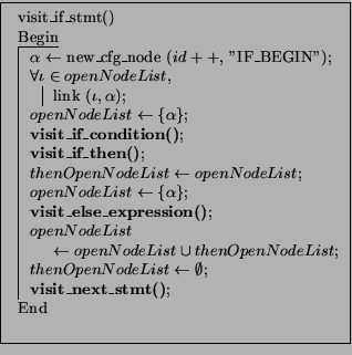
Now, we can see on Figure 15 the algorithm corresponding to an "if" statment. In the case of "if" statement, we need another list which is local to the algorithm to store the contents of the openNodeList after the visit of the "then". The beginning of the algorithm is very similar to the one used for expression. So, there is the creation of a node &alpha. Before calling the visitor for "then" branch, we initialize openNodeList with it. When the visit of the first branch of the "if" statment is finished, we store the state of open nodes in the thenOpenNodeList and initialize the list of open nodes to &alpha . Thus, we can visit the second branch of the "if" statement. When the visit is done, the list of open nodes becomes the union between itself and thenOpenNodeList. The thenOpenNodeList is then initialized to an empty set. Now, we can continue by visiting the next statement.
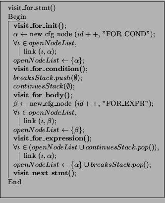
The algorithm (Figure 16) used when visiting a "for" statement is almost identical to the algorithm used for a "while" statement. The unique difference is after the visit of the body. Whereas in the while algorithm the link between basic block was done after the visit of the body, in the "for" statement, we need to visit the condition of the "for" before making those link. Other things are identical. We make a simplification by considering that the condition is a simple expression. We don't consider complex expression. We could've been inspired by the algorithm proposed in [4] but, it will be a part of our future work.
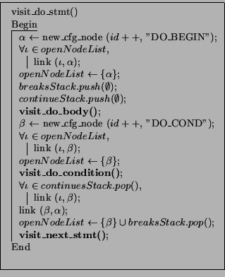
The extraction of the CFG for "do" statement is a little bit different than precedently. Like the other one, we started the algorithm (see Figure 17) with the creation of a basic block named DO_BEGIN, and, we link nodes in openNodeList to it. Let this node be &alpha. Before visiting the body of the statement, we push a new state at the top of breaks stack and continue stacks. When the body is visited, the next visit will be the condition of the do statement. So, we create a new node &beta and, we link all open nodes to this node. We add &beta in the list of open nodes and we can visit the condition of the "do". When this part is done, we link nodes contained in the openNodeList to &beta and, as the condition can have two different path (wrong or true), we link &beta to &alpha and, the openNodeList become the union between &beta and breaksStack.pop.
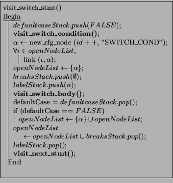
The particularity of the "switch" statement is that we can have a default case or not. To deal with this particularity, we use again a stack which will contain a boolean (see Figure 18). It's value is FALSE if there is no default case. Thus, at the beginning, like we don't know if there is a default case, we push a boolean FALSE on the stack. Between the condition of the "switch" and the body of the "switch" (which contains all case), the algorithm is like the other one. The difference here is after the visit of the body. We test if the top of the defaultcaseStack is TRUE or FALSE and, depending of the value, the initialisation of the open nodes will be different. If there is no default case, we need to add the node created at the beginning of the algorithm to the openNodeList, else, we do nothing. Now that the case of the default value is resolved, the list of the open nodes is set to the union of openNodeList and breaksStack.pop. Before calling the visitor for the next statement, we pop the label stack.
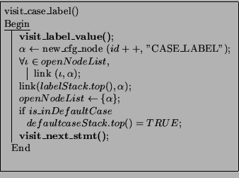
As we have seen it, the body of the "switch" is a whole of "case". Now, we will explain the algorithm used when we visit a case label (see Figure 19). This algorithm is simple and just refers to the description done for expression algorithm (see Figure 13) for details. The difference is the test of the default case. Thus, the treatement is basic and, if we are in a default case, we need to initialize the top of the defaultcaseStack to TRUE. For gasta, we know we are in a default case because the ASG has a different representation of this kind of node. A typical "case" has two tags, one is "next:" and the other one is "low :". If it's a default case, there will be only the tag "next:" because the "low :" represents the value of the label and of course, the default is by definition all values. So, the presence of a "low :" tag indicate that it's not a default case.
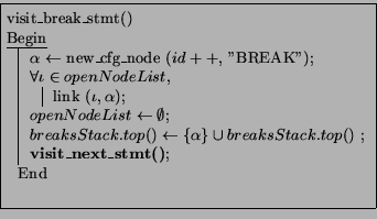
The treatement of "break" statement on Figure 20 is very straightforward. The only thing to do is adding the new basic block on top of the breaks stack and, initialize the openNodeList to empty set.
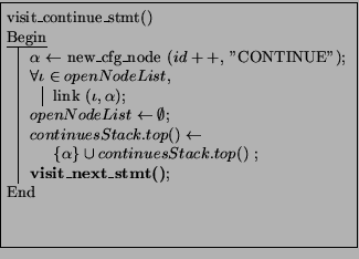
The "continue" statement is very similar to the "break" statement. The difference is obviously the node &alpha that we put on the continues stack instead of breaks state. The algorithm is describe on Figure 21.
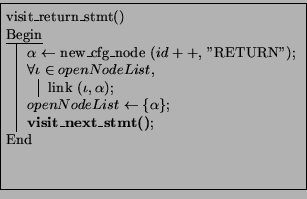
The algorithm (see Figure 22) used for "return" is exactly the same as this used for general expression. Here we can discuss about the initialization of the openNodeList to &alpha. Normally, the return has no successors because by definition, openNodeList is the list which contains a whole of nodes of which we are calculating the successors, however, "return" doesn't have any one (here we talk about intraprocedural analysis [3]). Nevertheless we decided to add it to openNodeList because the ASG generated by gcc has to return statement. Only one interests us but, we decided to keep both of them. To difference this needed by our analysis, we have two choices. Either we look the tags associated with the "return" statement, either we took the first one and ignore the second one because the usefull node is always before the useless (it is visited first). If we choose to test the tags, we must keep the return which have a tag "next:".
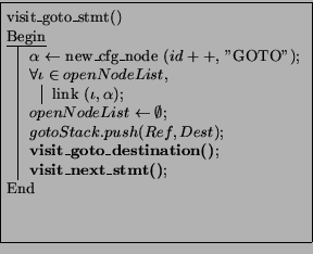
The analysis done for "goto" statement is different because we don't know what destination is reached by the "goto" until we reach the end of the code. Indeed, nothing prevents us to put a "label" stement just before the last line of code. So, the algorithm (shown Figure 23) keep each goto destination in a table and, with the destination we also keep a pointer to the node corresponding to the "goto" in the CFG. Thus, when the visit will be complete, we will go through this structure and, according to information found inside, we will link each "goto" with the corresponding "label". Like we will see in the next algorithm 24, label are store in a hash table and the key is the node number inside the ASG (the "goto" destination corresponds to this node number). Besides that every think else in the algorithm is like we saw in the precedents.
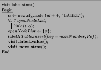
As we started to discuss it, we use a hash table to store informations needed by "goto" to link the node with is destination. As we can see on Figure 24, the key is the node number of the "label" in the ASG. The key gives an entry in the hash table which is a pointer to the "label" node in the CFG. So, if we have a "goto" statement with @53 as destination, we can find a pointer to the corresponding "label" in the CFG by given the key @53 and thus, we can link the "goto" to its "label".